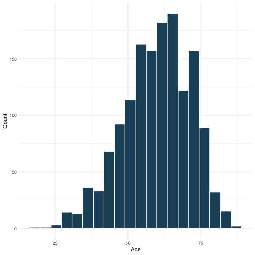
class: title-slide, center, middle <span class="fa-stack fa-4x"> <i class="fa fa-circle fa-stack-2x" style="color: #ffffffcc;"></i> <strong class="fa-stack-1x" style="color:#3b4245;">03</strong> </span> # Graphics for Communication ## R Markdown for Medicine ### Alison Hill · RStudio #### [rmd4medicine.netlify.com/](https://rmd4medicine.netlify.com/) --- class: middle, center # <i class="fas fa-cloud"></i> # Go here and log in (free): https://rstd.io/rmd4medicine-cloud --- layout: true <div class="my-footer"><span>https://rstd.io/rmd4medicine-cloud</span></div> --- exclude: true at this point, we should be within a bookdown with html and word doc output options? Or an rticles with bookdown under the hood? --- class: inverse, middle .pull-left[ <!-- --> ] -- .pull-right[ [`ggplot2` package](https://ggplot2.tidyverse.org/) [`ggplot2` cheatsheet](https://github.com/rstudio/cheatsheets/blob/master/data-visualization-2.1.pdf) [R4DS chapter](https://r4ds.had.co.nz/data-visualisation.html) ] --- class: middle, center, inverse <span class="fa-stack fa-4x"> <i class="fa fa-circle fa-stack-2x" style="color: #fff;"></i> <strong class="fa-stack-1x" style="color:#2f5275;">1 </strong> </span> # Get figures in --- class: your-turn # Your turn: Part 1 of 2 **WARM-UP**: open `03-draft.Rmd` and read the source file. It has several figures coded using the `ggplot2` package. 1. Knit the document to the `bookdown::html_document2` format — behold! 1. Add output options to this format to use one of the [bootswatch themes](https://rmarkdown.rstudio.com/docs/reference/html_document.html) and include a [floating table of contents](https://rmarkdown.rstudio.com/docs/reference/html_document.html#floating-table-of-contents). *(hint: `?html_document`)* 1. Knit to `bookdown::word_document2` (no options)- how does it look? 1. Add `distill::distill_article` as an output format (consider adding a TOC too) and knit- what differences do you see between this and the `bookdown::html_document2` format? _psst...next slide has answers..._ <div class="countdown" id="timer_5d7d4a9f" style="right:0;bottom:0;" data-warnwhen="0"> <code class="countdown-time"><span class="countdown-digits minutes">05</span><span class="countdown-digits colon">:</span><span class="countdown-digits seconds">00</span></code> </div> --- class: your-turn # Answer .pull-left[ ```yaml --- output: bookdown::html_document2: theme: flatly toc: true toc_float: true bookdown::word_document2: default distill::distill_article: toc: true --- ``` ] .pull-right[ ```` ```{r setup, include=FALSE} knitr::opts_chunk$set( echo = FALSE, warning = FALSE, message = FALSE, comment = NA, R.options = list(width = 70) ) ``` ```` Distill is much less chatty than other outputs due to default `knitr` code chunk options: https://rstudio.github.io/distill/basics.html#code-blocks ] --- class: middle, center # The line-up <img src="03-graphics_files/figure-html/unnamed-chunk-4-1.png" width="25%" /><img src="03-graphics_files/figure-html/unnamed-chunk-4-2.png" width="25%" /><img src="03-graphics_files/figure-html/unnamed-chunk-4-3.png" width="25%" /><img src="03-graphics_files/figure-html/unnamed-chunk-4-4.png" width="25%" /> --- # Including plots .pull-left[ ```r # PLOT: Age distribution ------------------------------------------------------- ggplot(mockdata, aes(age)) + geom_histogram(color = 'white', fill = scico(1, begin = .3, palette = "berlin"), bins = 20) + labs(x = "Age", y = "Count") + scale_y_continuous( breaks = scales::pretty_breaks() ) ``` Will this print? ] -- .pull-right[ <!-- --> ] --- # Including plots .pull-left[ ```r # PLOT: Age distribution ------------------------------------------------------- age_histogram <- ggplot(mockdata, aes(age)) + geom_histogram(color = 'white', fill = scico(1, begin = .3, palette = "berlin"), bins = 20) + labs(x = "Age", y = "Count") + scale_y_continuous( breaks = scales::pretty_breaks() ) ``` What about this? ] -- .pull-right[ ] --- # Including plots .pull-left[ ```r # PLOT: Age distribution ------------------------------------------------------- age_histogram <- ggplot(mockdata, aes(age)) + geom_histogram(color = 'white', fill = scico(1, begin = .3, palette = "berlin"), bins = 20) + labs(x = "Age", y = "Count") + scale_y_continuous( breaks = scales::pretty_breaks() ) age_histogram ``` ] -- .pull-right[ <!-- --> ] ??? so, how did we get a figure into R Markdown? Answer: it has to print! --- class: middle, center, inverse <span class="fa-stack fa-4x"> <i class="fa fa-circle fa-stack-2x" style="color: #fff;"></i> <strong class="fa-stack-1x" style="color:#2f5275;">2 </strong> </span> # Chunk options for plots --- # Chunk options for plots - fig resolution - fig size - [fig "device"](https://r4ds.had.co.nz/graphics-for-communication.html#other-important-options) .footnote[https://yihui.name/knitr/options/#plots] --- # Figure resolution .pull-left[ ```r # PLOT: Age distribution ------------------------------------------------------- age_histogram <- ggplot(mockdata, aes(age)) + geom_histogram(color = 'white', fill = scico(1, begin = .3, palette = "berlin"), bins = 20) + labs(x = "Age", y = "Count") + scale_y_continuous( breaks = scales::pretty_breaks() ) age_histogram ``` ] .pull-right[ <!-- --> ] --- # fig.retina .pull-left[ ```` ```{r} age_histogram ``` ```` <img src="03-graphics_files/figure-html/unnamed-chunk-10-1.png" width="70%" /> ] -- .pull-right[ ```` ```{r fig.retina=3} age_histogram ``` ```` <img src="03-graphics_files/figure-html/unnamed-chunk-11-1.png" width="70%" /> ] --- # out.width .pull-left[ ```` ```{r fig.retina=3, out.width="70%"} age_histogram ``` ```` <img src="03-graphics_files/figure-html/unnamed-chunk-12-1.png" width="70%" /> ] -- .pull-right[ ```` ```{r fig.retina=3, out.width="10%"} age_histogram ``` ```` <img src="03-graphics_files/figure-html/unnamed-chunk-13-1.png" width="10%" /> See also: + `fig.width` + `fig.height` + `fig.asp` https://r4ds.had.co.nz/graphics-for-communication.html#figure-sizing ] --- # fig.cap For the `ae_pct_plot`, I followed [these recommendations](https://www.bmj.com/content/355/bmj.i5078). ```` ```{r fig.cap="BMJ, 2016 paper", echo=FALSE} knitr::include_graphics(here::here("images/F3.large.jpg")) ``` ```` <div class="figure"> <img src="/Users/alison/rworkshops/rmd4medicine/static/slides/images/F3.large.jpg" alt="BMJ, 2016 paper" width="25%" /> <p class="caption">BMJ, 2016 paper</p> </div> ??? This is how you can also add static figures. You could use R Markdown, but with knitr you can also include a figure caption. As you might have noticed in your output, this ends up numbered. --- class: live-code # Live code demo We open up `03-draft.Rmd` and take the static image and together we: 1. Label that chunk 1. Add a cross-reference like `see Figure \@ref(fig:bmj)` 1. Try again with `counts-by-site` code chunk: `see Figure \@ref(fig:counts-by-site)` _(watch what happens if try to cross-reference without a caption!)_ .footnote[Cross-referencing only works in these output packages: distill, bookdown, blogdown] --- # Caption a figure ```` ```{r age-plot, echo=FALSE, fig.cap='Age distributions'} age_histogram ``` ```` .center[ <img src="03-graphics_files/figure-html/age-plot-1.png" width="25%" /> **Fig. 1:** Age distributions ] --- # Cross-reference a figure .pull-left[ See Figure `\@ref(fig:age-plot)`. ```` ```{r age-plot, echo=FALSE, fig.cap='Age distributions'} age_histogram ``` ```` ] .pull-right[ See Figure [1](). .center[ <div class="figure"> <img src="03-graphics_files/figure-html/unnamed-chunk-15-1.png" alt="Age distributions" width="70%" /> <p class="caption">Age distributions</p> </div> ] ] --- # Key takeaway Once you have: ✔️ A labeled chunk that produces a plot ✔️ A figure caption using `fig.cap` Then you can have: ### Cross-references!* .footnote[\* and you are using distill, bookdown, or blogdown output formats] --- class: your-turn # Your turn: Part 2 of 2 Now go through `03-draft-revised.Rmd` and read the source, then knit. .pull-left[ ```r # demographics----------------------------- age_density # multi-panel? <-ignore this age_boxplot # multi-panel? <-ignore this demo_tab # treatment response @ follow-up----------- surv_pct_plot # multi-panel? <-ignore this surv_days_plot # multi-panel? <-ignore this fu_tab # adverse events--------------------------- ae_pct_plot ae_tab ``` ] .pull-right[ 1. Add new code chunks containing tables and plots where you want. 1. Edit the code chunk options as you need to. 1. Add headers and other Markdown formatting as you see fit. 1. Feel free to add figure captions and in text cross-references. ] <div class="countdown" id="timer_5d7d4a07" style="right:0;bottom:0;" data-warnwhen="0"> <code class="countdown-time"><span class="countdown-digits minutes">05</span><span class="countdown-digits colon">:</span><span class="countdown-digits seconds">00</span></code> </div> --- class: middle, center, inverse <span class="fa-stack fa-4x"> <i class="fa fa-circle fa-stack-2x" style="color: #fff;"></i> <strong class="fa-stack-1x" style="color:#2f5275;">3 </strong> </span> # Combine figures in output --- # Arrange plots in a grid `cowplot::plot_grid()` for multi-panel plots .footnote[https://wilkelab.org/cowplot/articles/plot_grid.html] --- class: live-code # Live code demo We start with `03-draft-revised.Rmd` and combine `age_density` and `age_boxplot` with the `cowplot` package. ```r plot_grid(age_density, age_boxplot, labels = "AUTO") ``` <img src="03-graphics_files/figure-html/unnamed-chunk-18-1.png" width="70%" style="display: block; margin: auto;" /> --- class: your-turn # Your turn ## Make a plot grid Open up your `03-draft-revised.Rmd`. Combine `surv_pct_plot` and `surv_days_plot` with `cowplot::plot_grid()`. _psst...my answers on the next slide..._ <div class="countdown" id="timer_5d7d4bc3" style="right:0;bottom:0;" data-warnwhen="0"> <code class="countdown-time"><span class="countdown-digits minutes">03</span><span class="countdown-digits colon">:</span><span class="countdown-digits seconds">00</span></code> </div> --- class: your-turn # Answers ```` ```{r echo=FALSE, fig.retina=3, fig.asp=.5, fig.width=20} plot_grid(surv_pct_plot, surv_days_plot, labels = "AUTO") ``` ```` <img src="03-graphics_files/figure-html/unnamed-chunk-20-1.png" width="720" style="display: block; margin: auto;" /> --- class: middle, center, inverse <span class="fa-stack fa-4x"> <i class="fa fa-circle fa-stack-2x" style="color: #fff;"></i> <strong class="fa-stack-1x" style="color:#2f5275;">4 </strong> </span> # Get figures out --- # Exporting plots ```r ggsave() ``` --- # fig.path ```` ```{r ae-plot, fig.path="figs/", echo=FALSE} ae_pct_plot ``` ```` <img src="03-graphics_files/figure-html/ae-plot-1.png" width="70%" /> --- class: live-code # Live code demo We open up `03-draft-revised.Rmd` and together we: 1. Add `fig.path="figs/"` as a `knitr` code chunk option for a single plot _(watch what happens if we don't include the backslash!)_ 1. Knit and behold 1. We add a global `setup` chunk, if we have time. --- class: live-code # A global `setup` chunk One chunk to rule them all ```` ```{r setup, include = FALSE} knitr::opts_chunk$set( warning = FALSE, message = FALSE, echo = FALSE, fig.retina = 3, fig.path = here::here("alison-figs/") ) ``` ```` --- # ⭐ Tip http://zevross.com/blog/2017/06/19/tips-and-tricks-for-working-with-images-and-figures-in-r-markdown-documents/ <iframe src="http://zevross.com/blog/2017/06/19/tips-and-tricks-for-working-with-images-and-figures-in-r-markdown-documents/" width="100%" height="400px"></iframe> --- class: middle, center # ⏱ # Time for a break! <div class="countdown blink-colon noupdate-15" id="timer_5d7d4afd" style="right:0;bottom:0;" data-warnwhen="0"> <code class="countdown-time"><span class="countdown-digits minutes">10</span><span class="countdown-digits colon">:</span><span class="countdown-digits seconds">00</span></code> </div>